Modelling dissolved oxygen in rivers impacted by wastewater discharge
This learning module presents a model describing the concentration of dissolved oxygen in a river subjected to the input of oxygen-demanding waste. Students will use this model to illustrate how dissolved oxygen in a river responds to waste input and how to decide how much waste the river should be allowed to receive.
Municipal wastewater, when treated to quality standards determine by regulations, still contains low concentrations of oxygen-demanding organic compounds when discharged to receiving water bodies, typically streams or rivers. These organic compounds can be consumed by microorganisms within the river, but a concomitant oxygen consumption occurs as part of the microbial metabolism. If dissolved oxygen concentrations decrease too low, say 2-4 mg/L, some aquatic life such as fish cannot be supported. Thankfully, dissolved oxygen concentrations can be replenished by reaeration from the atmosphere. Though not the focus of this model, one may find small, man-made waterfalls near wastewater treatment system outlets to promote air-water mixing and consequently reaeration.
The properties and processes occurring in the river are as follows:
Advection: The flow of water downstream with velocity ux.
BOD loading: The concentration of oxygen-consuming waste in units of mg/L BOD (biochemical oxygen demand), which are analogous to mg/L dissolved oxygen. Wastewater discharge is mixed with the river water to an initial BOD concentration Lo.
Oxygen deficit: The river may already contain lower than saturation levels of dissolved oxygen, and the initial deficit (Do.) is the amount less than saturated concentration (saturated concentration, Csat, is typically near 9 mg/L dissolved oxygen).
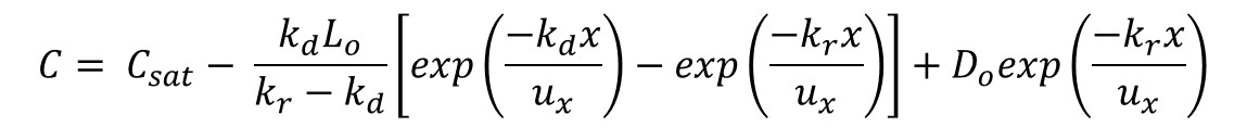
Oxygen consumption (decay): Dissolved oxygen (C) decays according to a first order reaction with rate coefficient kd, but its decay rate is also proportional to the amount of waste BOD still present which decays by a first order reaction as well, and so the overall dissolved oxygen decay rate is –kdLoexp(-kd t).
Oxygen reaeration: Dissolved oxygen in the river increases according to a first order reaction with rate coefficient kr. The rate expression is +kr(Csat – C).
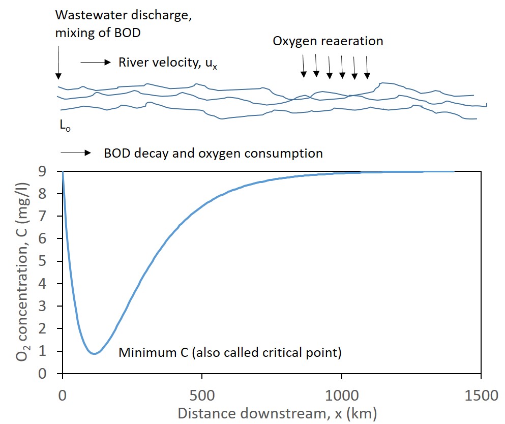
As the mixed water flows downstream, dissolved oxygen will decrease as it is consumed, but increase as the river becomes reaerated. The concentration of dissolved oxygen along the distance of the river can be described with the Streeter-Phelps equation:
A plot of C vs. x takes the shape of a “sag curve” where a minimum value of C occurs shortly after the input of wastewater. It is this minimum value of C and its location along the river that is of importance because they may indicate a condition of insufficient oxygen. Such a condition should be avoided by controlling the value of Lo for environmental conditions determining kd and kr. Using the spreadsheet, perform the following simulations.
Simulation 1: Using the pre-set condition in the spreadsheet, does the dissolved oxygen sag curve ever dip below 3 mg/L? If so, at what location downstream? At the moment, there is no initial dissolved oxygen deficit. If the initial deficit were to be 2 mg/L, would the minimum value of C decrease further?
Simulation 2: Using simulation 1 with the initial deficit of 2 mg/L, consider a different set of values for kd and kr in the wintertime, where water temperature is colder, microorganism metabolism is slower, and reaeration may be slightly faster. Adjust kd to a factor of 5 less, how does the curve change? Then, adjust kr to a factor of 2 more, does the curve still dip too far down?
Design 1: Using the condition arrived at the end of simulation 2, determine what Lo is the maximum amount that can be maintained while the minimum C value remains above 3 mg/L. This amount would determine how much BOD could be discharged from the wastewater treatment plant.
Design 2: A separate river has a velocity that is one tenth the velocity as in simulation 2 (all other parameters are as in simulation 2). Does the sag curve change the minimum C or its location? What is the maximum Lo that can be maintained in this situation?
This learning module was supported by resources from the National Science Foundation.