Modelling air pollution concentrations downwind from smokestack emissions
This learning module presents a model describing the concentration of an air pollutant in the form of a plume as it moves downwind and spreads out from a stack emission. Students will use this model to illustrate how pollutant concentrations at ground level are controlled by stack geometry and atmospheric conditions, and how to decide an appropriate stack height for public health.
Many industries release gaseous and particulate substances that can be classified as air pollutants and affect the quality of air. Example industries are coal-fired power plants that release carbon dioxide, sulfur dioxide, and particulate matter, and even manufacturing plants that release low concentrations of chemicals. When the emissions leave the stack, a few processes may happen:
Plume rise occurs when the emitted air carrying the pollutants rises to a height higher than the stack.
Advection occurs when the wind carries the pollutants downwind.
Dispersion occurs when the pollutants spread out horizontally and vertically as the wind transports them. This dispersion happens as pollutant molecules collide, causing them to move away from each other.
The anatomy of a typical stack emissions is as follows:
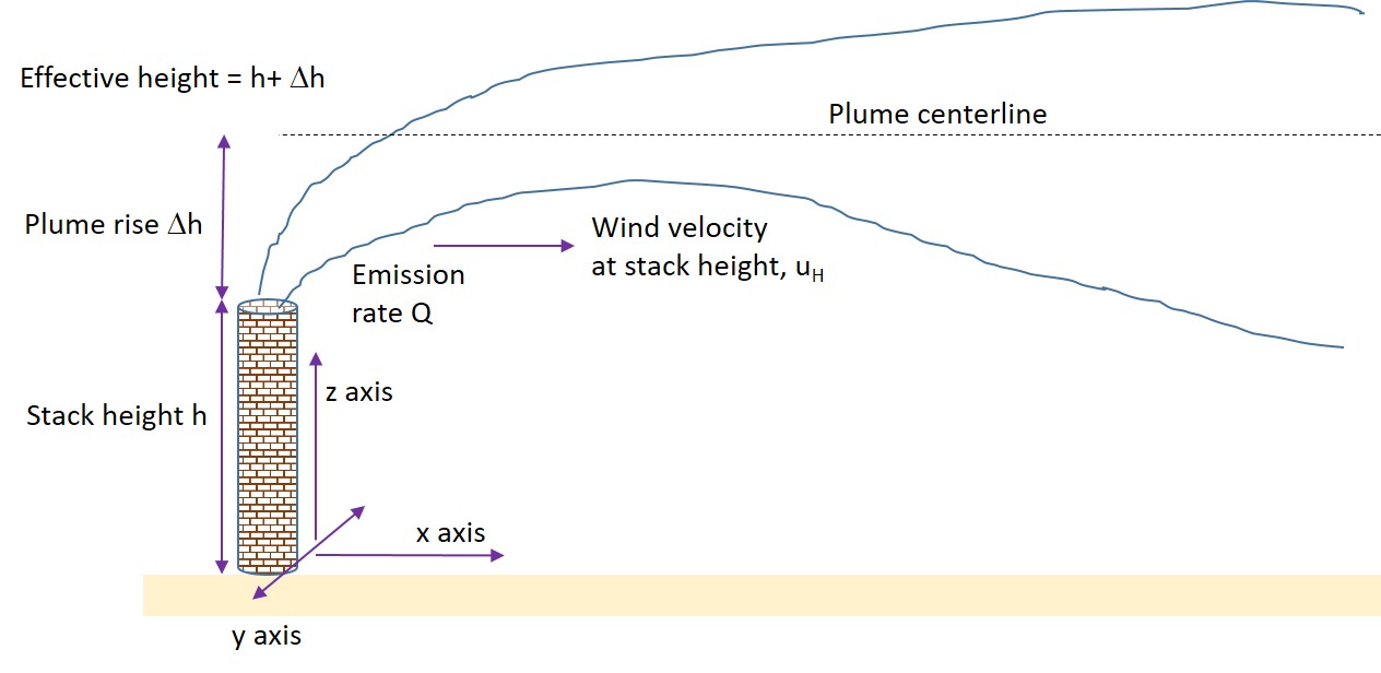
In addition to wind speed (at the stack height), the atmospheric conditions can be characterized by stability class (labeled A through F). The meanings of the stability classes are: A Very unstable, B Moderately unstable, C Slightly unstable, D Neutral, E Slightly stable, F Stable.
Stability refers to how well the air mass surrounding the stack is encouraged to not move up or down. An air mass that is well encouraged to move vertically is an unstable condition that can cause more movement of pollutants away from the ground level.
The plume shape takes on that similar to a cone with its point located above the stack and a spreading out downwind. The dispersion of pollutants horizontally and vertically is assumed to be described mathematically with a normal distribution, a bell curve where concentrations are higher in the middle (along the plume centerline) and decrease outwards towards the edges. To describe these normal distributions, the dispersion coefficients σy and σz are used. These values increase as distance downwind from the stack increases because the plume spreads out over greater distance. These values also differ for each stability class, with greater dispersion coefficients for more unstable conditions. The values of σy and σz are therefore a function of downwind distance x and can be described mathematically with equations from the scientific literature (McMullan 1975) .
The concentration of emitted pollutant can be calculated at any point (x, y, z) as follows:
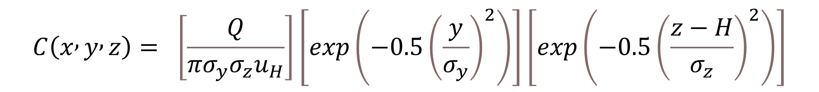
Note: Ground level pollutant concentrations are often the focus of investigations because more exposure to humans is possible. Along the plume centerline will have the greatest pollutant concentration and will also be of importance. In these cases, z=0 and y=0.
A plot of concentration versus distance x will provide a downwind concentration profile for any value of z and y. This plot can be programmed using the downloadable spreadsheet here. The plots take a typical shape of low concentrations immediately near the stack (because the plume has not reached the ground yet), higher concentrations downstream, followed by lower concentrations far away (due to significant dispersion). Using the spreadsheet, perform the following simulations by creating these plots.
Simulation 1: What is the effect of atmospheric stability on downwind, ground level concentrations along the plume centerline? Use a stack height of 80 m, a plume rise of 20 m, an emission rate of 0.5 g/s, and a wind speed of 2 m/s. Compare plume shapes for stability classes A through F. For each class, note the maximum downwind ground level concentration and the distance from the stack where it occurs. Comment on whether higher ground level concentrations are experienced at stable or unstable conditions.
Simulation 2: What is the effect of wind speed on ground level concentrations for each stability class? Use the conditions in simulation 1. Do windy days make for a ‘safer’ condition of lower concentrations at ground level?
Design 1: Design an appropriate stack height such that the maximum allowable downwind ground level concentration of pollutants does not exceed a regulatory amount of 1 microgram per cubic meter. The stack must satisfy this criteria for all stability classes and for all possible wind speeds of 1, 2, 3, and 4 m/s. The pollutant is emitted at a rate of 2 g/s. Typical plume rise is 10 m. This stack height will need to be designed later by structural engineers.
Design 2: A stack height is fixed and cannot be increased, but in this problem the stack will be emitting a different pollutant (after a different industrial process is activated) at a different emission rate. The anticipated emission rate is 3 g/s. The stack height is 100 m, plume rise 10 m, and wind speed 1, 2, 3, and 4 m/s. First, will the ground level concentration along the centerline ever exceed the regulatory standard of 2 micrograms per cubic meter for any stability class and wind speed? Second, determine an emission rate Q such that the 2 micrograms per cubic meter criteria is never exceeded for any stability class and wind speed combination. This final emission rate will have to be ensured later by engineers who will design ways to scrub the pollutant out of the waste stream to meet this required Q.
This learning module was supported by resources from the National Science Foundation.